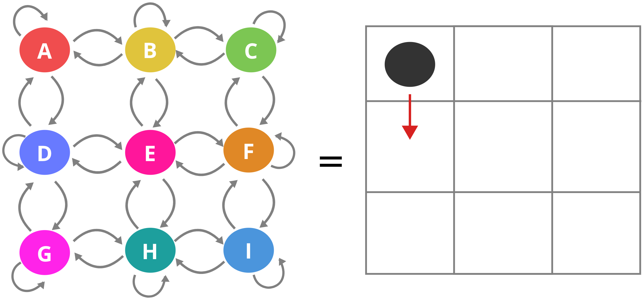
Hello Everyone!! in today’s post I thought of writing an introduction for Markov Chains. Simply put, Markov chains are used to model systems that change randomly where a current state is only dependent on the previous state.(I’ll explain what states are in a minute) In fact, its a pretty powerful technique used in fields ranging from computer networks to statistical physics. I’ll explain the basics of Markov chains using a simple example called the pebble game as illustrated above.
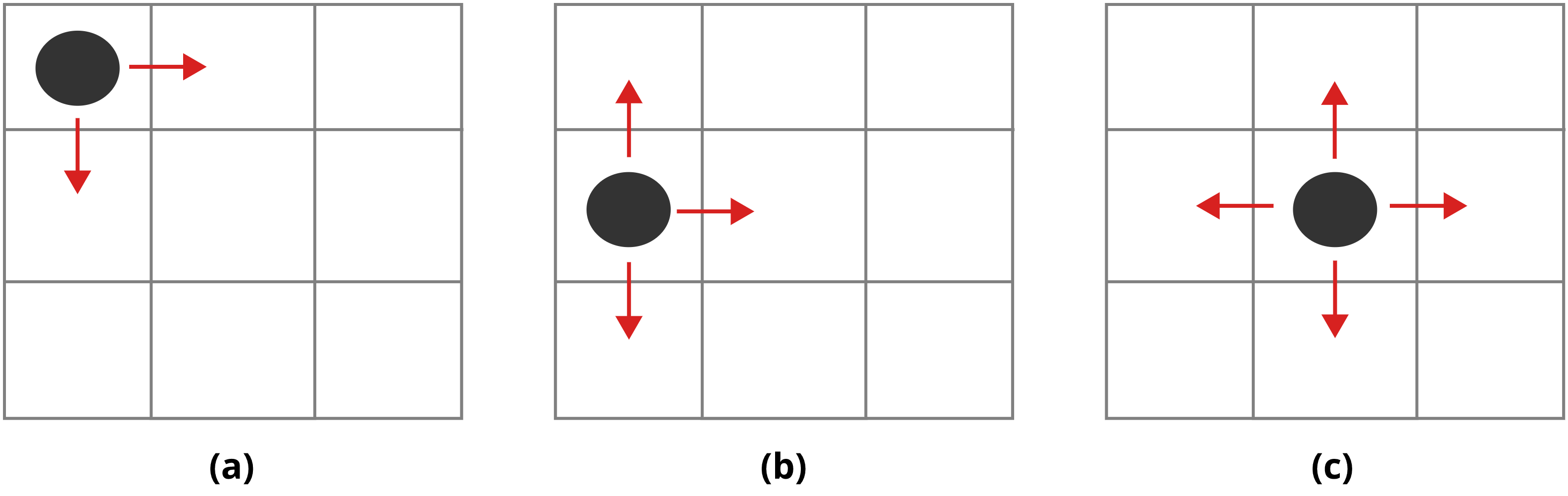
Now imagine we have a 3x3 grid just like the image above, with the black dot being a pebble. At each instance in time a person picks the pebble up and tries to throw to some other directly linked cell randomly.(Note that throwing the pebble to diagonal cells is not possible) The image below shows the three types of throws possible:
config (a) :The pebble is at the corner, So theres only two positions it can be thrown to.The pebble can’t be thrown up or to the left.config (b) :The pebble has three possible cells to be thrown to.The pebble can’t be thrown to the left.config (c) :The pebble can be thrown in all directions.
So the question is, lets say at each time step someone picks the pebble and throws to an adjacent cell and keeps on doing it. After 10,000 iterations of the process where would the pebble likely be? OR whats the probability of some cell having the pebble, provided this was done for a long time? Now intuitively since there are 9 cells, and the person is going to keep on throwing the pebble in this space for a long time we can make a guess that the probability of finding this pebble in any cell is equally likely, i.e the probability will be \(\frac{1}{9}\). This is actually the correct result, but there might be problems so complex that getting these sort of insights might not be as intuitive, and that’s where this technique truly shines.
There are two main steps in defining Markovian models, the 1st is to define the states & the second is to populate whats called a transition matrix. Both of which I’ll go through below.
States
Before diving into the technique itself, there are some things called states that must be defined.
States refer to all the possible configurations of the system.
In our example, states refer to the cell position of the pebble at a given time instance. If you look at the figure again I’ve drawn an image with circles labeled A-I, these labels refer to the different cell locations the pebble could be in. Furthermore, I’ve also drawn arrows, these arrows represent the possible transitions from one state(cell) to another. That image corresponds to all the possible things that could happen in this system of ours, and by definition nothing beyond those transitions should occur.
Lets take the initial state A, from this location if the pebble is to be thrown there are three possibilities,
- A transition from A to B
- A transition from A to D
- No throw is possible up or to the left, therefore a transition from A to A
Similarly, the image represents all transitions in all states whom fall under the basic configurations explained in (a), (b) & (c). Note that it’s impossible to throw the pebble from A to E or from A to F, so there is no arrow corresponding to that.
Figuring out the states of your problem is the hard part. Because there is not a set way in defining those, and it all comes down to how you see the problem. As you’ll see in the section below what comes after that is way more simpler.
The transition matrix
Now that we have our states defined, the second problem is the transitions. It’s all nice that our figure has arrows pointing to what might happen next. But which of those possibilities actually happen? The thing to remember here is our entire system evolves randomly with time. Any of the state transitions could happen at some instance. Therefore the transitions aren’t deterministic rather they are probabilistic. Meaning there is a probability value associated with each transition from one state to another.
Ok, now how do we get those probabilities. First of all since the throws are done randomly and independently of each other. config (c) shows the best possible case where a pebble could be thrown in all four directions. Since any of these transitions is equally likely, The probability of moving from state E to either F, B, D, H is \(\frac{1}{4}\) (\(P_{EF} = P_{EB} = P_{ED} = P_{EH} = \frac{1}{4}\)). However, when considering configs (a) & (b) the pebble cannot be thrown in all directions. Therefore the probabilities for those impossible throws gets added on to a special transition probability namely \(P_{AA},~P_{DD}\) and vice-versa. According to this logic the probabilities for config (a) & (b) would be \(P_{AA}=\frac{1}{2},~P_{AB}=P_{AD}=\frac{1}{4}\) and \(P_{DD} = P_{DA} = P_{DE} = P_{DG} = \frac{1}{4}\) respectively. All these probability values can be represented in matrix form, and that’s called a transition matrix(\(\mathbb{P}\)).
\begin{equation} \mathbb{P}=\begin{pmatrix} P_{AA} & P_{AB} & P_{AC} & P_{AD} & P_{AE} & P_{AF} & P_{AG} & P_{AH} & P_{AI} \\ P_{BA} & P_{BB} & P_{BC} & P_{BD} & P_{BE} & P_{BF} & P_{BG} & P_{BH} & P_{BI} \\ P_{CA} & P_{CB} & P_{CC} & P_{CD} & P_{CE} & P_{CF} & P_{CG} & P_{CH} & P_{CI} \\ P_{DA} & P_{DB} & P_{DC} & P_{DD} & P_{DE} & P_{DF} & P_{DG} & P_{DH} & P_{DI} \\ P_{EA} & P_{EB} & P_{EC} & P_{ED} & P_{EE} & P_{EF} & P_{EG} & P_{EH} & P_{EI} \\ P_{FA} & P_{FB} & P_{FC} & P_{FD} & P_{FE} & P_{FF} & P_{FG} & P_{FH} & P_{FI} \\ P_{GA} & P_{GB} & P_{GC} & P_{GD} & P_{GE} & P_{GF} & P_{GG} & P_{GH} & P_{GI} \\ P_{HA} & P_{HB} & P_{HC} & P_{HD} & P_{HE} & P_{HF} & P_{HG} & P_{HH} & P_{HI} \\ P_{IA} & P_{IB} & P_{IC} & P_{ID} & P_{IE} & P_{IF} & P_{IG} & P_{IH} & P_{II} \\ \end{pmatrix}\
\end{equation} By substitution of values, \begin{equation} \mathbb{P}=\begin{pmatrix} \frac{1}{2} & \frac{1}{4} & 0 & \frac{1}{4} & 0 & 0 & 0 & 0 & 0 \\ \frac{1}{4} & \frac{1}{4} & \frac{1}{4} & 0 & \frac{1}{4} & 0 & 0 & 0 & 0 \\ 0 & \frac{1}{4} & \frac{1}{2} & 0 & 0 & \frac{1}{4} & 0 & 0 & 0 \\ \frac{1}{4} & 0 & 0 & \frac{1}{4} & \frac{1}{4} & 0 & \frac{1}{4} & 0 & 0 \\ 0 & \frac{1}{4} & 0 & \frac{1}{4} & 0 & \frac{1}{4} & 0 & \frac{1}{4} & 0 \\ 0 & 0 & \frac{1}{4} & 0 & \frac{1}{4} & \frac{1}{4} & 0 & 0 & \frac{1}{4} \\ 0 & 0 & 0 & \frac{1}{4} & 0 & 0 & \frac{1}{2} & \frac{1}{4} & 0 \\ 0 & 0 & 0 & 0 & \frac{1}{4} & 0 & \frac{1}{4} & \frac{1}{4} & \frac{1}{4} \\ 0 & 0 & 0 & 0 & 0 & \frac{1}{4} & 0 & \frac{1}{4} & \frac{1}{2} \\ \end{pmatrix} \end{equation}
Note that the summation of probabilities at each row equals to 1 & for transitions that aren’t possible the value in the matrix is 0. Now that we have this matrix we can use it to calculate the probabilities of being in some state after a given set of iterations. lets consider \(\alpha_{t}\) as the probability distribution of the pebble at time t. i.e \(\alpha_{t} = (P_A,P_B,P_C,P_D,P_E,P_F,P_G,P_H,P_I)\). Therefore at t=0, since the pebble is at state A, \(\alpha_{t=0}=(1,0,0,0,0,0,0,0,0)\).
The following method is used to calculate the probability distribution at some t.
\[\alpha_{t} = \alpha_{t-1}.\mathbb{P}\]
Then for t=1, \begin{aligned} \alpha_{t=1} &= \alpha_{t=0}. \mathbb{P} \
\alpha_{t=1} &=(1~0~0~0~0~0~0~0~0).\begin{pmatrix} \frac{1}{2} & \frac{1}{4} & 0 & \frac{1}{4} & 0 & 0 & 0 & 0 & 0 \\ \frac{1}{4} & \frac{1}{4} & \frac{1}{4} & 0 & \frac{1}{4} & 0 & 0 & 0 & 0 \\ 0 & \frac{1}{4} & \frac{1}{2} & 0 & 0 & \frac{1}{4} & 0 & 0 & 0 \\ \frac{1}{4} & 0 & 0 & \frac{1}{4} & \frac{1}{4} & 0 & \frac{1}{4} & 0 & 0 \\ 0 & \frac{1}{4} & 0 & \frac{1}{4} & 0 & \frac{1}{4} & 0 & \frac{1}{4} & 0 \\ 0 & 0 & \frac{1}{4} & 0 & \frac{1}{4} & \frac{1}{4} & 0 & 0 & \frac{1}{4} \\ 0 & 0 & 0 & \frac{1}{4} & 0 & 0 & \frac{1}{2} & \frac{1}{4} & 0 \\ 0 & 0 & 0 & 0 & \frac{1}{4} & 0 & \frac{1}{4} & \frac{1}{4} & \frac{1}{4} \\ 0 & 0 & 0 & 0 & 0 & \frac{1}{4} & 0 & \frac{1}{4} & \frac{1}{2} \\ \end{pmatrix} \
\alpha_{t=1} &=(\frac{1}{2}~\frac{1}{4}~0~\frac{1}{4}~0~0~0~0~0) \end{aligned}
Similarly, this process can be carried out for any given number of steps. Now, what about our earlier guess of \(\frac{1}{9}\) . This value is called the steady state probability value. By definition it’s the probability of being in a specific state provided that infinitely many iterations have taken place. The easiest way to obtain that is to convolve the equation above many times over OR simply computing a large power of \(\mathbb{P}\). Therefore simply \(\mathbb{P}^{x\rightarrow\infty}=\frac{1}{9}\) for all the states. So there you go, a somewhat simple introduction to Markov Chains. If you want to learn more about this I highly recommend the book Introduction to Probability Models.
So until next time,
Cheers!
Next: Finding cycles in linked lists
Prev: Proving correctness of Algorithms